Sensor group: Merge physical sensors into one virtual sensor

Applies to

Sensoft Multiline

Issue

Can I use two 1-axis sensors like one 2-axis sensor, i.e. creating just one spool file? Does it work also with 3 or 4 axes?

Solution

Yes. You can group two or more physical sensors into one virtual one:

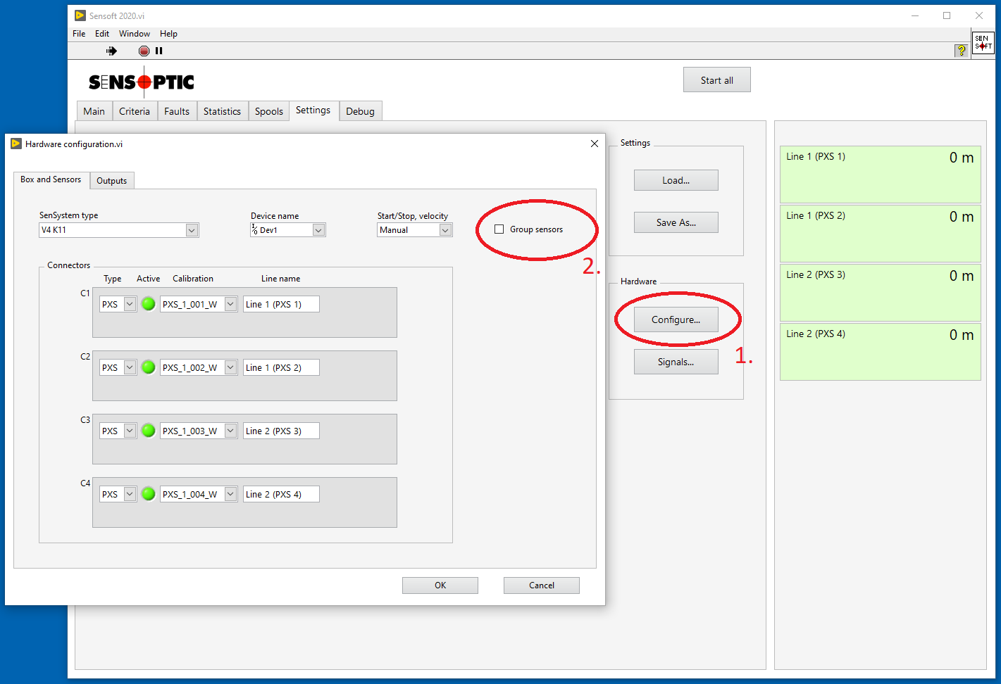
1. In the Sensoft software go to page Settings and click on Configure... to enter in the Hardware configuration dialog window (Figure 1). Each line is a physical sensor.
2. Click on Group sensors.
   

   Figure 1: Hardware configuration dialog window. This and the following figures illustrate a setup consisting of two filaments each being measured by two PXS sensors. This figure shows the situation without sensor groups: Each sensor generates its file, so that for each spool two files are created.

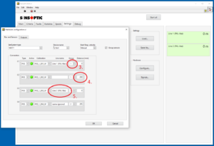
   Figure 2: Same setup as in Figure 1, but with grouped sensors. The first two sensors, assumed along the same wire, distant 200 mm and rotated 90° respect to each other, are grouped. Also the other two sensors are grouped. After accepting the changed settings by closing the dialog window with OK, Sensoft Multiline (rear window in the figure) will show just two lines and thus save one file for each spool.

3. New fields appear (Figure 2). Assign the same Group number to each sensor you want to link together. In Sensoft Multiline the sensor with the same Group will be merged into a single line (Figure 2, rear window). The grouped sensors should be of the same Type.
4. In the other new field Distance [mm] enter the distance between the sensors measured along the wire. The first sensor of the group a defect on the wire encounters should have distance zero, and the last sensor of the group it encounters the greatest distance. The distance should be measured from the slit of the first sensor of the group to the respective slit. Distance is used to synchronize the sensors within a group so that a defect is seen from all sensor at the same position.
5. The Line name of the top-most sensor in the group in Hardware configuration will give the Line name of the merged sensor as it appears in Sensoft Multiline (Figure 2). The line names of the other sensors in the group are ignored.
6. Accept by pressing OK and save the settings.

You can also link 3 or more physical sensors in one group. With mono-axial sensors there will be measurements along 3 or more axes, with bi-axial sensors along 6 or more axes. Relevant for finding defects are the aggregated signals, calculated by merging the signals from all axes.

The following table shows how the aggregated signals are calculated in grouped sensors:

where Max, Min and (arithmetic) Mean are taken over all axes.

The ordering of the axes of the combined sensor (i.e. which will be the x-axis and so forth) is determined by which connectors the physical sensors are attached to the Sensystem. The axes of the combined sensor will be the axes of the sensor at with lower connector number followed by the axes of the sensor with the next-lower connector number, and so forth. E.g., if group 1 is composed of a mono-axial PXS sensor connected to connector C1 and another PXS sensor connected to C2, the combined sensor has C1 as x-axis and C2 as y-axis. As another example, if group 2 is composed of a bi-axial PXL sensor connected to connector C3 and another PXL sensor connected to C4, the combined sensor has as x-axis the x-axis of the PXL connected to C3, as y-axis the y-axis of C3, as  third and forth axis the axes of C4. Note that only defects along the first two axes of the combined sensor can be detected separately from the other axes, by using criteria like  Warning if LU x > 50 µm  and  Warning if LU y > 50 µm. 

Notes

Note 1: In the case of exactly 2 axes with "Wire" calibration (i.e. Calibration ends with "_W"): LU = LU x + LU y  and NE = NE x + NE y. The reasons are to calculate it like our current bi-axial sensors and because it does a better job with blisters in the hidden zones.

When working with grouped sensors it is important that distance between the grouped sensors (Distance [mm]) is as short as possible and that the filament velocity is as stable as possible. If the velocity is not stable, or if it is set incorrectly on page Criteria, the signals of the sensors do not align well and a single fault may appear as a pair of faults. The tolerable velocity offset (in %) is approximately 2.5 * Velocity [m/min] / Distance mm] . E.g., with velocity 200 m/min and distance 200 mm, we have a tolerable velocity error of 2.5%, or 5 m/min. Beyond that, double faults may appear and in the case of Note 1, small blisters may pass undetected. This easy rule hold for the default settings and is derived in Note 2.

Note 2: With the default settings, there are signal points every 1 ms, and two peaks are thus undiscernible if they have Δt < 1.5 ms. Mathematically Δt = Δ(s/v) = s*v^-2*Δv = s/v * Δv/v , where s is Distance and v is Velocity. Therefore Δv/v = Δt*v/s < 1.5 ms * v/s = 1.5*100/60 * (v in m/min)/(s in mm) %.