Maximum velocity of the filament

Applies to

Sensoft Multiline

Question

What is the maximal allowed velocity of the filament?

Answer

One has to differentiate between two cases: whether one measures just the fault size, or also the fault length and profile. Basically, the first case is faster and usable up to 1500 m/min, the second only up to approximately 50 m/min.

Fault size

You are using this method if you are using the keywords lump or neck-down in your criteria, e.g. in Alarm if lump > 10 µm.

The maximal velocity v_max of the filament is:

v_max = W × f_c

where W is the slit width of the sensor and f_c the cut-off frequency of a low-pass filter used in the sensor. For typical values W = 0.35 mm and f_c = 70 kHz we have v_max = 1470 m/min. You can calculate your value using this link. Please contact us, if you need the parameters of your sensor or if you need higher velocity, which can be achieved with sensors optimized for high velocity.

Let us understand where the above equation comes from. In this case faults are detected by measuring an analog lump signal. The signal left by a long fault passing at high velocity is equal to that of a shorter fault passing at some lower velocity. Therefore the filament velocity is only limited by the shortest fault that should be detected, which has the length of about the slit width of the sensor. The formula relating v_max and f_c is complicated, but approximately (and conservatively) we have that the signal duration t ≈ W / v_max ≈ 1 / f_c . Note that v_max is not a digital boundary, but means that at velocities over v_max the measured size of short faults starts getting attenuated.

Fault size, length and profile

You are using this method if you are using the keywords  LU x,  LU y,  Lump  or  Neck-down  in your criteria.

The maximal velocity v_max of the filament is:

v_max = W × f / M

where W is the slit width of the sensor, f the Data rate [Hz] specified on page Settings of Sensoft Multiline and M a noise-dependent factor typically equal to 16. The maximal value for the data rate f is f_tot / (n_S × n_A), i.e. the total data rate f_tot of the Sensystem (400 kHz for the Sensystem Standard, 250 kHz for Sensystem Compact and Sensystem Process) divided by the number n_S of used lines (i.e. activated sensors) and the number n_A of axes per sensor. For a Sensystem Standard with four bi-axial sensors we thus get f = 50 kHz.

With M = 16, slit width W = 0.25 mm and f = 50 kHz we get a maximal velocity v_max of about 45 m/min. You can calculate your value using this link. Please contact us if you intend to measure fault length and profile.

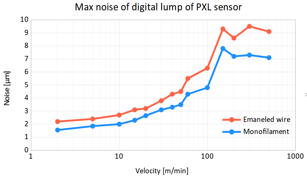
Figure 1: Noise of digital lump signal versus velocity for a PXL sensor (PXL 2.068 with mask 10 x 0.25 mm) at Data rate = 50 kHz.

Details on M and derivation of the equation above. The factor M tells how many times we have to reduce our data, to achieve the noise level we wish. Without data reduction (M = 1), the equation is  v_max = W × f  and the derivation is as in the previous chapter.

Figure 1 shows the measured noise for a PXL sensor as a function of velocity. One clearly sees that the noise increases with velocity, since less and less averaging can be done, until it goes to a plateau where no average is possible. In the Enameled wire case (red curve) the lump signal is calculated as Lump = LU x + LU y, while in the Monofilament case (blue curve) as Lump = max(LU x, LU y), see how faults are measured. The enameled wire case thus adds the noise of the two axes, resulting in about 30% higher noise than the monofilament case. A mono-axial sensor, such as a PXS, closely follows the monofilament case. Note that the monofilament case is also used with rectangular enameled wires, since blisters on each face are assumed independent. The noise in Figure 1 is measured as maximum lump signal in 1 m when there is no wire, and the used Data rate is 50 kHz. This means that it is what you see in the Mean graph on page Statistics if you measure with Mean data interval 1 m.

Figure 2: Maximum noise of digital lump signal versus velocity for a PSD sensor (PSD 5.001 with mask 2 x 0.35 mm) at Data rate = 50 kHz.

Figure 2 shows the same measurements for the PSD sensor.

These two graphs show the noise for Data rate = 50 kHz, but since the noise depends only on M, they let you calculate it also for other values of Data rate. Basically at half Data rate you can go only half as fast. E.g.: A Data rate = 25 kHz the noise at 10 m/min is equal to the noise at 20 m/min with Data rate = 50 kHz and same slit width.